Gradient Descent

1. Introduction

1.1. Why do we need GD?

We can easily find the prediction function from a given dataset using the formula of linear regression:

\hat{\mathbf{x}} = (A^TA)^{-1}A^T\mathbf{b}

However, since it involves an inverse function, it is manageable with small datasets and low dimensions, but when dealing with larger datasets and higher dimensions, it consumes a lot of computational resources. Therefore, we need to use Gradient Descent, a classic yet very popular algorithm today.

Or when finding the extremum of a function, the equation $f'(x)=0$ cannot be solved easily. In this case, we can use the gradient descent algorithm to find an approximate solution.

1.2 Method

Gradient Descent is a first-order iterative optimization algorithm for finding a local extremum of a differentiable function. To find a local minimum of a function using gradient descent, one takes steps proportional to the negative of the gradient (or approximate gradient) of the function at the current point. Conversely, taking steps proportional to the positive of the gradient leads to finding a local maximum; this method is called gradient ascent.

More specifically, GD repeatedly changes the value of $x \; (x := x + \beta)$ so that in each iteration, it is hoped that $f(x)$ becomes smaller and approaches the minimum.

The way to adjust $\beta$ and ensure $f(x)$ decreases is to set $\beta$ to a negative portion of the gradient: $\beta = -\alpha f'(x)$ , where $\alpha$ is a positive number called the learning rate. Finally, we get:

\begin{align*} x := x - \alpha f'(x) \end{align*}

According to Figure 1, at point $x_0$ we have $f'(x_{0}) < 0 \Rightarrow \alpha f'(x_{0}) < 0$ , which means the value of $x$ will increase or move to the right, causing the value of $f(x)$ to gradually decrease towards the minimum.

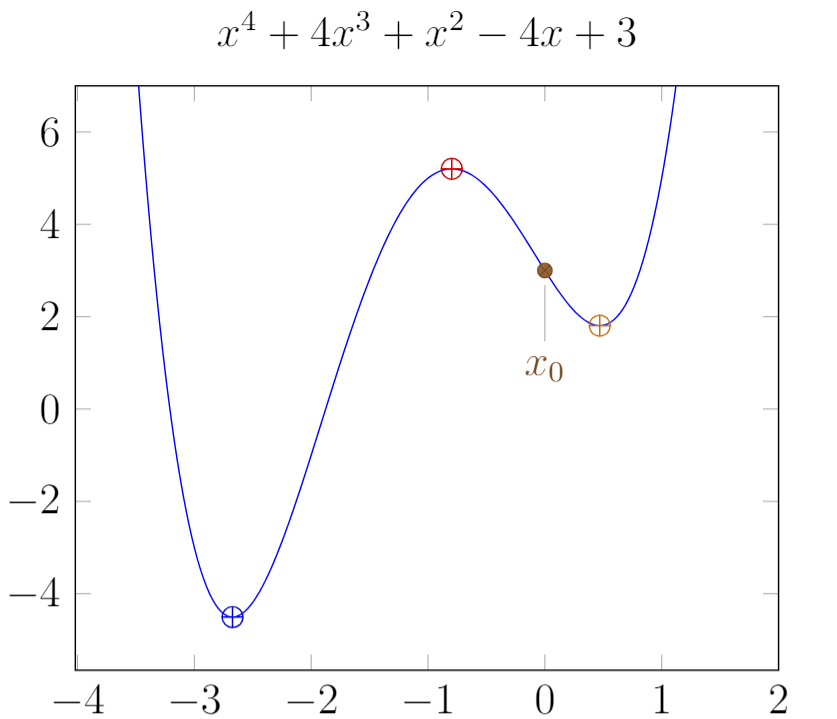
Figure 1: Gradient Descent Diagram

2. Gradient Descent and Linear Regression.

Now let's go through the concept of matrix derivatives (to work with multi-dimensional data) and numerical differentiation (to calculate the approximate gradient at a specific value of $x$ ).

2.1 Matrix Derivatives

In the previous example, $x$ was just a one-dimensional vector, but in reality, the problems presented can also have $x$ as a vector in $n$ -dimensional space.

In linear regression, $x$ is a vector, and its derivative formula is:

\triangledown_x f(x) = \begin{bmatrix} \frac{\partial f}{\partial x_{1}}\newline \vdots \newline \frac{\partial f}{\partial x_{m}} \end{bmatrix}\tag{1}

2.2 Numerical Differentiation

According to numerical differentiation, we can calculate the derivative according to (3) with a small error compared to the normal formula (2).

We will use it to check if we have calculated the derivative correctly.

\begin{aligned} f’(x) = \lim_{\varepsilon \rightarrow 0}\frac{f(x + \varepsilon) - f(x)}{\varepsilon} \end{aligned}\tag{2}

\begin{aligned} f’(x) \approx \frac{f(x + \varepsilon) - f(x - \varepsilon)}{2\varepsilon} \end{aligned}\tag{3}

You can read more here: Numerical Differentiation - Wikipedia

2.3 Simulation with Python

Summarizing the Linear Regression problem. First, consider the following two sets:

X = [x_{1}, x_{2}, ... , x_{m}]^{T} \\ Y = [y_{1}, y_{2}, ... , y_{m}]^{T}

We need to find $a$ and $b$ to have the equation:

Y \approx a + bX

In other words:

\begin{aligned} \begin{bmatrix} y_{1}\\ y_{2}\\ \vdots \\ y_{m} \end{bmatrix} \approx \begin{bmatrix} 1 & x_{1} & x_{1}^{2} \dotsm & x_{1}^{n - 1}\\ 1 & x_{2} & x_{2}^{2} \dotsm & x_{2}^{n - 1} \\ \vdots & \vdots & \vdots & \vdots \\ 1 & x_{m} & x_{m}^{2} \dotsm & x_{m}^{n - 1} \end{bmatrix} \cdot \begin{bmatrix} a_{1}\\ a_{2} \\ \vdots \\ a_{n} \end{bmatrix} \Leftrightarrow Y \approx Ax \end{aligned}\tag{4}

But there are no $a,b$ that satisfy creating a line passing through all the data points, so we will find $a,b$ such that:

\begin{aligned} f(x) = \left \| Ax - Y \right \|^2_{2} \; min \end{aligned}\tag{5}

The derivative of (5) with respect to $x$ is:

\begin{equation} f'(x) = 2.A^{T} . \left | Ax - Y \right | \end{equation}\tag{6}

Figure 2: Gradient Descent Animation

gradient_descent.py

from matplotlib import animation
from matplotlib.animation import writers
import numpy as np
import matplotlib
import matplotlib.pyplot as plt
from sklearn import linear_model

def cost(x):
  m = A.shape[0]
  return 0.5/m * np.linalg.norm(A.dot(x) - b, 2)**2

def grad(x):
  m = A.shape[0]
  return 1/m * A.T.dot(A.dot(x) - b)

def numerical_grad(x):
  eps = 1e-4
  g = np.zeros_like(x)
  for i in range(len(x)):
      x1 = x.copy()
      x2 = x.copy()
      x1[i] += eps
      x2[i] -= eps
      g[i] = (cost(x1) - cost(x2))/(2*eps)
  return g

def check_grad(x):
  x = np.random.rand(x.shape[0], x.shape[1])
  grad1 = grad(x)
  grad2 = numerical_grad(x)
  if np.linalg.norm(grad1 - grad2) > 1e-5:
      print("Check grad function!")
  return

def gradient_descent(x_init, learning_rate, iteration):
  x_list = [x_init]
  for i in range(iteration):
      x_new = x_list[-1] - learning_rate*grad(x_list[-1])
      if np.linalg.norm(grad(x_new))/len(x_init) < 1e-3:
          break
      x_list.append(x_new)
  return x_list

A = [2,9,7,9,11,16,25,23,22,29,29,35,37,40,46]
A = np.array([A]).T # Ox
b = [2,3,4,5,6,7,8,9,10,11,12,13,14,15,16]
b = np.array([b]).T # Oy

# Draw data
fig1 = plt.figure("GD for Linear Regression")
ax = plt.axes(xlim=(-10,60), ylim=(0, 20))
plt.plot(A, b, 'ro')

# Linear Regression
lr = linear_model.LinearRegression()
lr.fit(A,b)
x0_gd = np.linspace(1,46,2)
y0_sklearn = lr.intercept_[0] + lr.coef_[0][0]*x0_gd
plt.plot(x0_gd, y0_sklearn, color="green")

# Add one to A
ones = np.ones((A.shape[0], 1), dtype=np.int8)
A = np.concatenate((ones, A), axis=1)

# Random and plot initial line
x_init = np.array([[1.], [2.]]) # (a, b)
y0_init = x_init[0][0] + x_init[1][0]*x0_gd # y = a + bx
plt.plot(x0_gd, y0_init, color="black")
# check grad
check_grad(x_init)

# Run
iteration = 100
learning_rate = 0.0001
x_list = gradient_descent(x_init, learning_rate, iteration)

for i in range(len(x_list)):
    y0_gd = x_list[i][0] + x_list[i][1]*x0_gd
    plt.plot(x0_gd, y0_gd, color="black", alpha=0.3)

line , = ax.plot([],[], color="blue")
def update(i):
    plt.xlabel('Iteration: {}   Learning rate: {}'.format(len(x_list) - 1, learning_rate))
    y0_gd = x_list[i][0][0] + x_list[i][1][0]*x0_gd
    line.set_data(x0_gd, y0_gd)
    return line,

iters = np.arange(0,len(x_list), 1)

plt.legend(('Data', 'Solution by Linear Regression', 'Initial Line For GD'), loc=(0.48, 0.01))
plt.title("Gradient Descent")
line_ani = animation.FuncAnimation(fig1, update, iters, interval=50, blit=True)

plt.show()

3. Going into more detail

3.1 When to stop?

The relationship between the number of changes in $x$ (Iteration) and the value of $f(x)$ (Cost Value) Figure 3.1. It is easy to see that the Cost Value tends to approach $0$ and remains stable after iteration 50. Repeating the remaining iterations does not seem to reduce the Cost Value much and may not be necessary.

Based on this, we can come up with a good threshold to stop the GD function.

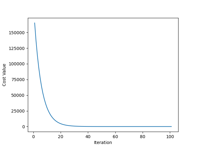
Figure 3.1: The relationship between cost and iteration

Figure 3.2: Case $n= 3$ or quadratic function (Parabolic)

Figure 3.2 shows that when the threshold of the gradient value is around $0.02$ ( $|Grad|< 0.02$ ), we get a relatively good result compared to the result from Linear Regression.

gradient_descent_2.py

import numpy as np
import matplotlib.animation as animation
import matplotlib.pyplot as plt
from matplotlib.animation import writers
def cost(x):
    m = A.shape[0]
    return 0.5/m * np.linalg.norm(A.dot(x) - b)**2

def grad(x):
    m = A.shape[0]
    return 1/m * A.T.dot(A.dot(x) - b) # return f'(x):[a, b, c].T

def numerical_grad(x):
    eps = 1e-4
    g = np.zeros_like(x)
    for i in range(len(x)):
        x1 = x.copy()
        x2 = x.copy()
        x1[i] += eps
        x2[i] -= eps
        g[i] = (cost(x1) - cost(x2))/(2*eps)
    return g

def check_grad(x):
    g1 = grad(x)
    g2 = numerical_grad(x)
    if np.linalg.norm(g1 - g2) > 1e-5:
        print("Check grad function")
    return

def gradient_descent(x_random, learning_rate, iteration):
    x_list = [x_random]
    for i in range(iteration):
        x_new = x_list[-1] - learning_rate*grad(x_list[-1])
        if np.linalg.norm(grad(x_new))/len(x_gd) < 0.03:
            break
        x_list.append(x_new)
    return x_list

b = [2,5,7,9,11,16,19,23,22,29,29,35,37,40,46,42,39,31,30,28,20,15,10,6]
b = np.array([b]).T
A = [2,3,4,5,6,7,8,9,10,11,12,13,14,15,16,17,18,19,20,21,22,23,24,25]
x_gd = np.linspace(1,46,10000)
# x_random = np.random.rand(3, 1)
# print(x_random)
x_random = np.array([[ -2.1],
       [ 5.1],
       [-2.1]])
fig1 = plt.figure("GD for Linear Regression")
ax = plt.axes(xlim=(-5,30), ylim=(-5, 50))

A = np.array([A]).T
plt.plot(A,b, 'ro')
# add ones and col 3 to A
ones = np.ones((A.shape[0], 1), dtype=np.int8)
col_3 = A*A
A = np.concatenate((ones, A, col_3), axis=1)

# Linear Regression
x_lg = np.linalg.inv(A.T.dot(A)).dot(A.T.dot(b))
y_lg = x_lg[0][0] + x_lg[1][0]*x_gd + x_lg[2][0]*x_gd*x_gd
plt.plot(x_gd, y_lg, color="green")

# Plot random
y_random = x_random[0][0]  + x_random[1][0]*x_gd + x_random[2][0]*x_gd*x_gd
plt.plot(x_gd, y_random, color="black")
# check grad
check_grad(x_random)

iteration = 70
learning_rate = 0.000001

x_list = gradient_descent(x_random, learning_rate, iteration)
for i in range(len(x_list)):
    y0_gd = x_list[i][0] + x_list[i][1]*x_gd + x_list[i][2]*x_gd*x_gd
    plt.plot(x_gd, y0_gd, color="black", alpha=0.3)

# Draw animation
line , = ax.plot([],[], color="blue")
def update(i):
    y0_gd = x_list[i][0][0] + x_list[i][1][0]*x_gd + x_list[i][2][0]*x_gd*x_gd
    line.set_data(x_gd, y0_gd)
    return line,

iters = np.arange(0,len(x_list), 1)
# Legend for plot
plt.xlabel('Iteration: {}   Learning rate: {}  |Grad| = {}'.format(len(x_list) - 1, learning_rate, np.linalg.norm(grad(x_list[-1]))/len(x_gd)))
plt.legend(('Data', 'Solution by Linear Regression', 'Initial Line For GD'), loc=(0.48, 0.01))
plt.title("Gradient Descent")
line_ani = animation.FuncAnimation(fig1, update, iters, interval=50, blit=True)

# Save animation to gif file
# Writer = writers['ffmpeg']
# writer = Writer(fps=15, metadata={'artist': 'Me'}, bitrate=1800)

# line_ani.save('GA Animation.gif', writer)

# fig2 = plt.figure()
# print(len(x_list))
# cost_list = []
# iteration_list = []
# plt.xlabel("Iteration")
# plt.ylabel("Cost Value")
# for i in range(len(x_list)):
#     iteration_list.append(i+1)
#     cost_list.append(cost(x_list[i]))
# plt.plot(iteration_list, cost_list)

plt.show()

3.2. Stuck at local minima

When randomly initializing $x$ and running, as mentioned above, there will be many local minima. Random initialization can cause us to get stuck at local minima, not the global minimum, as shown in Figure 4, resulting in a non-optimal solution. When working with higher-dimensional spaces, there are even more local minima.

Figure 4: Stuck at local minima

3.3. Learning Rate

The learning rate ( $\alpha$ ) is a very important parameter. A small $\alpha$ as in Figure 5 can slow down GD and make it very slow to converge. On the other hand, a large $\alpha$ as in Figure 5 can make GD unable to converge.

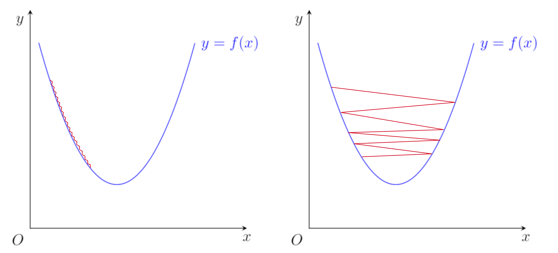
Figure 5: Learning Rate (left: small $\alpha$ , right: big $\alpha$ )

4. Conclusion

Gradient Descent is a very popular and powerful optimization method. It can help us find the extrema of a function quickly and efficiently. However, choosing the learning rate and the initial point is an important issue that needs to be carefully considered.